
Artificial Intelligence - How to measure performance - Accuracy, Precision, Recall, F1, ROC, RMSE, F-Test and R-Squared

We currently see a lot of AI algorithms being created, but how can we actually measure the performance of these models? What are the terms we should look at to detect this?
These are the questions I would like to tackle in this article. Starting from "Classification models" where we will look at metrics such as Accuracy, Precision, Recall, F1 Score and the ROC curve towards "regression models" where we will tackle the Root Mean Squared Error, F-Test and R-Squared methods.
Performance in Classification Models
Often when we are reading through papers on the internet, we see a table popping up that looks like this:
||Accuracy|Precision|Recall|F1| |-|-|-|-|-| |BTE|0.75|0.76|0.84|0.80| |CRF|0.82|0.88|0.81|0.84| |…|…|…|…|…| |Web2Text|0.86|0.87|0.90|0.88|
Note: Numbers taken from the Web2Text slides.
But what do these actually mean? Well let us take a deeper look at the different terms, starting of with introducing the "Confusion Matrix".
Confusion Matrix
A key concept that we need to know before being able to explain the performance metrics is the confusion matrix.
Definition: A confusion matrix is a table that is often used to describe the performance of a classification model (or "classifier") on a set of test data for which the true values are known.
A confusion matrix will look like this:
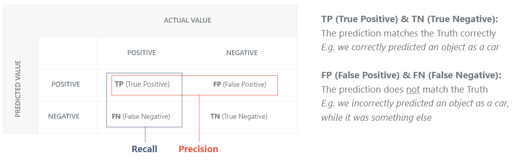
The above might look "confusing" but is actually quite simple. The top line dictates the "Actual Value (=truth)" while the left side shows the "prediction".
We could look at this in the sense of that whenever we predict correctly we will see "True", while as we predict wrongly we will see "False" correlated to the actual value Positive or Negative
Mapping this to the terms filled in:
- True Positive: Prediction = True, Truth = True
- False Positive: Prediction = True, Truth = False
- False Negative: Prediction = False, Truth = True
- True Negative: Prediction = False, Truth = False
Let's look at an example to make this more clearer.
Example: "We want to show the confusion matrix for a classifier that classifies if an object recognition model detected an object as a car or not". Then we could see the following confusion matrix for 1.000 test cases:
||Positive|Negative| |-:|:-:|:-:| |Positive|330 (TP)|2 (FN)| |Negative|7 (FP)|661 (TN)|
Showing that we correctly identified a car in 330 cases, wrongly detected a car 2 times, correctly predicted that it was not a car 661 times and wrongly predicted that it was not a car 7 times.
Or in other words: We were wrong 9 times and correct 991 times (also known as accuracy, but more about this later).
Accuracy
In short: Accuracy is how well the model performs
Formula: (TP + TN) / (TP + TN + FP + FN) or #CORRECT_PREDICTIONS / #TOTAL
Precision
In short: How often are we correct in our positive prediction?
Formula: (TP) / (TP + FP) or #CORRECT_POSITIVE_PREDICTIONS / #POSITIVE_SAMPLES
With Precision we want to make sure that we can accurately say when it should be positive. E.g. in our example above we want to make sure that when we say that it's car, that it really is a car and not some other object. This is important since we will often take actions based on our detections (e.g. in a self-driving car we could change the speed based on this).
Recall
In short: How often did we wrongly classify something as not true (= false)?
Formula: (TP) / (TP + FN) or #CORRECT_POSITIVE_PREDICTIONS / #TRUE_TRUTH_VALUES
Recall highlights the cost of predicting something wrongly. E.g. in our example of the car, when we wrongly identify it as not a car, we might end up in hitting the car.
F1 Score
In short: Utilize the precision and recall to create a test's accuracy through the "harmonic mean". It focuses on the on the left-bottom to right-top diagonal in the Confusion Matrix.
Formula: 2 * ((Precision * Recall) / (Precision + Recall))
Looking at the definitions of Precision and Recall, we can see that they both focus on high impact cases (e.g. we don't want to crash cars when we detected wrongly as not a car (= FN) and we don't want to say that it's a car if it's not (= FP)). This is what the F1 score does, it will focus on what impacts our business the most compared to the Accuracy score.
In other terms, we can thus say that the F1 score focuses on the left-bottom to right-top diagonal.
ROC Curve
In short: This curve allows us to select the optimal model and discard sub-optimal ones.
Formula: False Positive Rate (FPR) = X-Axis and True Positive Rate (TPR) = Y-Axis
- FPR:
TP / (TP + FN) - TPR:
FP / (FP + TN)
The ROC Curve (= Receiver Operating Characteristic) shows the performance, while the "AUC (= Area Under the Curve)" performance metric allows us to describe this as a value to measure the performance of classification models.
Every time when we classify a point, we take the probability being returned to state if it's matching or classifier or not (e.g. is it a car or not). But to be able to return true or false, we now have to introduce a threshold that will convert this probability into a classification.
Based on the threshold selected, we will be able to construct a confusion matrix.
We will now discretize the range of our threshold value (e.g. we make our range of [0, 1] to [0.0, 0.1, 0.2, …, 0.9, 1.0]) which we can now create the respective confusion matrices for. With those confusion matrices we will now calculate the True Positive Rate (= TPR) through the formula TPR = TP / (FP + TN) and the False Positive Rate (= FPR) through FPR = TP / (TP + FN) and plot these.
This eventually will result in something as this:
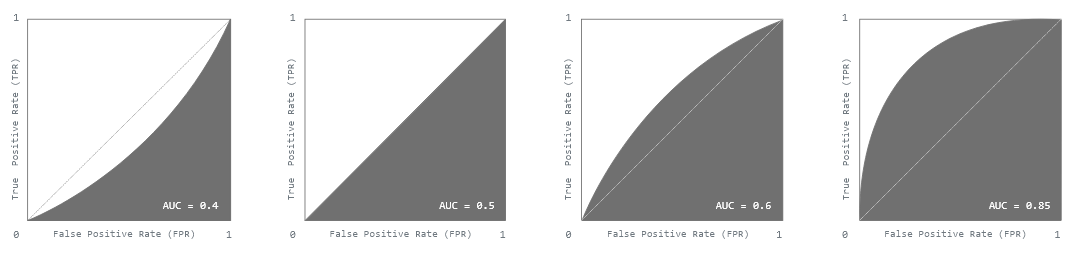
Note: We strive to have a model that has a high AUC value, or a ROC curve that shows as much to the left top as possible.
Performance in Regression Models
To calculate the performance of regression models, we utilize mathematical formulas that will compare the plotted graph to the points that we are predicting.
A good regression model should focus on minimizing the difference between the observation and the predicted value, while being unbiased. (Unbiased means that we try to find a balance between over-estimation and under-estimation)
Root Mean Square Error (RMSE)
This is simply the root of the Mean Square Error:
$$ RMSE = \sqrt{\sum^n{i=1}\frac{(\hat{y}i - y_i)^2}{n}} $$
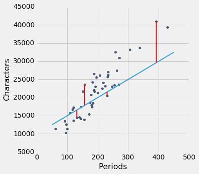
Which translates to taking the distance between the actual point and the predicted point, squaring this and then dividing by the amount of points we have for the mean.
Graphically this look like:
F-Test
In short: The F-Test is used to compare statistical models that were fitted to a dataset, it allows us to identify the model that best fits the population.
Formula: $F = \frac{explained variance}{unexplained variance}$
- Explained Variance: $\sum^K{i=1}ni\frac{(\bar{Y}_i - \bar{Y})^2}{K - 1}$
- Unexplained Variance: $\sum^K{i=1} \sum^{ni}{j=1} \frac{(Y{ij} - \bar{Y}_i)^2}{N - K}$
- K = Number of groups
- N = Overall Sample Size
- $Y_{ij}$ = $j^{th}$ observation in the $i^{th}$ out of $K$ groups
- $\bar{Y}$ = Overall mean of the data
R-Squared
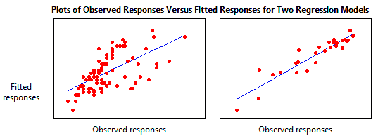
In short: R-Squared describes how well a model fits for a linear regression model. The higher R, the better the fit.
Formula: $R2 = 1 - \frac{Explained Variation}{Total Variation} = 1 - \frac{SS{res}}{SS_{tot}}$
- $\hat{y} = \frac{1}{n} \sum^n{i = 1} yi$ (the mean of the observed data)
- $SS{tot}$: $\sumi(y_i - \hat{y})^2$ (total sum of squares)
- $SS{res}$: $\sumi(yi - fi)^2$ (sum of squares of residuals)
The below picture illustrates:
- $SS_{tot}$: red
- $SS_{res}$: blue

R-Squared (or also called the "Coefficient of Determination") will show how close the data is to the fitted regression line. Or in other words, It indicates the percentage of the variance in the dependent variable that the independent variables explain collectively.
This is an interesting metric, because it allows us to understand better if our model is being overfitted or not.


Comments ()