
Facebook's Open-Source Reinforcement Learning Platform - A Deep Dive

Facebook decided to open-source the platform that they created to solve end-to-end Reinforcement Learning problems at the scale they are working on. So of course I just had to try this ;) Let's go through this together on how they installed it and what you should do to get this working yourself.
I started by creating a brand new installation of Ubuntu 18.10 Also tested and verified working on Windows Subsystem for Linux
Installing Anaconda
Let's start by installing Anaconda, this is easily done by navigating to the documentation located at https://conda.io/docs/user-guide/install/index.html whereafter we can find the link to the Linux Installer https://www.anaconda.com/download/#linux which will give us the installer script: https://repo.anaconda.com/archive/Anaconda3-5.3.0-Linux-x86_64.sh.
We can download and run this by running:
curl https://repo.anaconda.com/archive/Anaconda3-5.3.0-Linux-x86_64.sh -o conda.sh
bash conda.sh
Then follow the steps of the installer to install Anaconda
Once you did this, add the conda installation to your PATH variable through:
echo 'export PATH="$PATH":/home/<YOUR_USER>/anaconda3/bin' >> ~/.bashrc
. ~/.bashrc
Note: the default installation of anaconda is /home/ubuntu/anaconda3 for the Python 3 version
Configuring Anaconda for our Horizon Installation
Facebook Horizon requires several channels for certain software which we can easily add to anaconda:
conda config --add channels conda-forge # ONNX/tensorboardX
conda config --add channels pytorch
Installing Horizon
For a deeper dive on how you can install Horizon, check out the Git repo: https://github.com/facebookresearch/Horizon/blob/master/docs/installation.md
git clone https://github.com/facebookresearch/Horizon.git
cd Horizon/
conda install `cat docker/requirements.txt` # wait till it solved the environment, then select y
source activate base # Activate the base conda environment

pip install onnx # Install ONNX
export JAVA_HOME="$(dirname $(dirname -- `which conda`))" # Set JAVA_HOME to anaconda installation
cd # Go back to root

# Install Spark 2.3.1
wget http://www-eu.apache.org/dist/spark/spark-2.3.1/spark-2.3.1-bin-hadoop2.7.tgz
tar -xzf spark-2.3.1-bin-hadoop2.7.tgz
sudo mv spark-2.3.1-bin-hadoop2.7 /usr/local/spark

export PATH=$PATH:/usr/local/spark/bin # add to PATH so we can find spark-submit

# Install OpenAI Gym
pip install "gym[classic_control,box2d,atari]"

# Build Thrift Classes
cd Horizon/
thrift --gen py --out . ml/rl/thrift/core.thrift

# Build Horizon
pip install -e . # we use "-e" for "ephemral package" which will instantly reflect changes in the package
Horizon (Global Overview)
Introduction
Horizon is an End-To-End platform which "includes workflows for simulated environments as well as a distributed platform for preprocessing, training, and exporting models in production." - (Source)
From reading the paper we can read that this platform was created with the following in mind:
- Ability to Handle Large Datasets Efficiently
- Ability to Preprocess Data Automatically & Efficiently
- Competitive Algorithmic Performance
- Algorithm Performance Estimates before Launch
- Flexible Model Serving in Production
- Platform Reliability
Which sounds awesome to me, so let's get started by how we are able to utilize this platform, whereafter we can do a more deep-dive in how it works.
For some of the terminology used in Reinforcement Learning, feel free to check my previous blog post about it.
Getting Started
Getting started with Horizon is as easy as checking the usage documentation written by them. This includes the steps
- Creating training data
- Converting the data to the timeline format
- Create the normalization parameters
- Train the model
- Evaluate the model
Horizon - Batch RL (Deep-Dive)
Now we know what the general idea of the Horizon platform is, let's run through the different steps as written in the usage document and deep-dive on them, discovering what is going on behind the scenes. Let's start by creating our training data.
1. Creating Training Data
Our usage document lists that we should create the training data through these commands:
# Create a directory where we will put the training data
mkdir cartpole_discrete

# Generate training data
python ml/rl/test/gym/run_gym.py -p ml/rl/test/gym/discrete_dqn_cartpole_v0_100_eps.json -f cartpole_discrete/training_data.json
but what does this actually do? Opening up the run_gym.py file located in ml/rl/test/gym/ shows us the following in the main() method:
def main(args):
    parser = argparse.ArgumentParser(
        description="Train a RL net to play in an OpenAI Gym environment."
    )
    parser.add_argument("-p", "--parameters", help="Path to JSON parameters file.")
Which shows us that when running the command python ml/rl/test/gym/run_gym.py that we are able to see the usage of our script in the console, running this results in:
Traceback (most recent call last):
  File "ml/rl/test/gym/run_gym.py", line 611, in <module>
    + " [-s <score_bar>] [-g <gpu_id>] [-l <log_level>] [-f <filename>]"
Exception: Usage: python run_gym.py -p <parameters_file> [-s <score_bar>] [-g <gpu_id>] [-l <log_level>] [-f <filename>]
Explaining us that if we give the parameter file defined by our -p parameter it will load this JSON file and load it into a variable called params, while if we add the -f parameter, we will be able to save the collected samples as an RLDataSet to the provided file.
main() Method
The main method will now continue doing a couple of things:
# Load our parameters from the json
with open(args.parameters, "r") as f:
    params = json.load(f)

# Initialize a dataset variable of type `RLDataset` if the `file_path` parameter is set
#    `file_path`: If set, save all collected samples as an RLDataset to this file.
dataset = RLDataset(args.file_path) if args.file_path else None

# Call the method `run_gym` with the parameters and arguments provided
reward_history, timestep_history, trainer, predictor = run_gym(
    params, args.score_bar, args.gpu_id, dataset, args.start_saving_from_episode
)

# Save our dataset if provided through the -f parameter
if dataset:
    dataset.save()

#  Save the results to a csv if the `results_file_path` parameter is set
if args.results_file_path:
    write_lists_to_csv(args.results_file_path, reward_history, timestep_history)

# Return our reward history
return reward_history
After running our command shown in the usage document python ml/rl/test/gym/run_gym.py -p ml/rl/test/gym/discrete_dqn_cartpole_v0_100_eps.json -f cartpole_discrete/training_data.json we can see the following structure in the training_data.json file which was defined by the -f parameter.
{
    "ds": "2019-01-01",
    "mdp_id": "0",
    "sequence_number": 10,
    "state_features": {
        "0": -0.032091656679586175,
        "1": -0.016310561477682117,
        "2": -0.01312794549150956,
        "3": -0.04438365281404494
    },
    "action": "1",
    "reward": 1.0,
    "action_probability": 1.0,
    "possible_actions": [
        "0",
        "1"
    ],
    "metrics": {
        "reward": 1.0
    }
}
RLDataset Class
This is generated by the -f parameter that will be saving the results in a format provided by the RLDataset class to the file provided. Checking this class located at ml/rl/training/rl_dataset.py shows us:
"""
Holds a collection of RL samples in the "pre-timeline" format.

:param file_path: String Load/save the dataset from/to this file.
"""

# === LINES REMOVED ===

self.rows.append(
{
    "ds": "2019-01-01",  # Fix ds for simplicity in open source examples
    "mdp_id": str(mdp_id),
    "sequence_number": int(sequence_number),
    "state_features": state_features,
    "action": action,
    "reward": reward,
    "action_probability": action_probability,
    "possible_actions": possible_actions,
    "metrics": {"reward": reward},
}
run_gym() Method
Now we can see that the lines are being created and saved in-memory in the RLDataset class. But what is actually using this and filling it in? Let's first take a look at our run_gym() method in general:
env_type = params["env"]

# Initialize the OpenAI Gym Environment
env = OpenAIGymEnvironment(
    env_type,
    rl_parameters.epsilon,
    rl_parameters.softmax_policy,
    rl_parameters.gamma,
)
replay_buffer = OpenAIGymMemoryPool(params["max_replay_memory_size"])
model_type = params["model_type"]

use_gpu = gpu_id != USE_CPU

# Use the "training" {} parameters and "model_type": "<MODEL>" model_type
# to create a trainer as the ones listed in /ml/rl/training/*_trainer.py
# The model_type is defined in /ml/rl/test/gym/open_ai_gym_environment.py
trainer = create_trainer(params["model_type"], params, rl_parameters, use_gpu, env)

# Create a GymDQNPredictor based on the ModelType and Trainer above
# This is located in /ml/rl/test/gym/gym_predictor.py
predictor = create_predictor(trainer, model_type, use_gpu)

c2_device = core.DeviceOption(
    caffe2_pb2.CUDA if use_gpu else caffe2_pb2.CPU, int(gpu_id)
)

# Train using SGD (stochastic gradient descent)
# This just passess the parameters given towards a method called train_gym_online_rl which will train our algorithm
return train_sgd(
    c2_device,
    env,
    replay_buffer,
    model_type,
    trainer,
    predictor,
    "{} test run".format(env_type),
    score_bar,
    **params["run_details"],
    save_timesteps_to_dataset=save_timesteps_to_dataset,
    start_saving_from_episode=start_saving_from_episode,
)
The run_gym method appears to be using the parameters that we loaded from our JSON file to initialize the OpenAI Gym Environment. So let's see how one of these JSON files look like by opening one, running a quick cat ml/rl/test/gym/discrete_dqn_cartpole_v0_100_eps.json shows us:
{
  "env": "CartPole-v0",
  "model_type": "pytorch_discrete_dqn",
  "max_replay_memory_size": 10000,
  "use_gpu": false,
  "rl": {
    "gamma": 0.99,
    "target_update_rate": 0.2,
    "reward_burnin": 1,
    "maxq_learning": 1,
    "epsilon": 1,
    "temperature": 0.35,
    "softmax_policy": 0
  },
  "rainbow": {
    "double_q_learning": false,
    "dueling_architecture": false
  },
  "training": {
    "layers": [
      -1,
      128,
      64,
      -1
    ],
    "activations": [
      "relu",
      "relu",
      "linear"
    ],
    "minibatch_size": 64,
    "learning_rate": 0.001,
    "optimizer": "ADAM",
    "lr_decay": 0.999,
    "use_noisy_linear_layers": false
  },
  "run_details": {
    "num_episodes": 100,
    "max_steps": 200,
    "train_every_ts": 1,
    "train_after_ts": 1,
    "test_every_ts": 2000,
    "test_after_ts": 1,
    "num_train_batches": 1,
    "avg_over_num_episodes": 100
  }
}
Which shows that the Environment, Epsilon, Softmax Policy and Gamma parameters are all used to boot op the OpenAIGymEnvironment with the remaining parameters being passed to the trainer. Next to that the run_gym method will also initialize a replay_buffer, create the trainer and create predictor. Whereafter it will run the train_sgd method.
Since we now know our run_gym() method, let's look further at how our dataset variable is passed further:
run_gym()will get the method passed by themain()method as thesave_timesteps_to_datasetparameterrun_gym()will pass this to thetrain_sgd()methodtrain_sgd()will pass it to thetrain_gym_online_rl()method.
traingymonline_rl() Method
When this parameter is now defined, the train_gym_online_rl() method will save several variables through the insert() method defined in the RLDataset class:
Remember that theRLDatasetclass was defined in the file:ml/rl/training/rl_dataset.pyTheinsertmethod is defined as:RLDataset::insert(mdp_id, sequence_number, state, action, reward, terminal, possible_actions, time_diff, action_probability)
Source: run_gym.py#L208
|Source Variable from run_gym.py|Output Variable|Type|Description| |-|-|-|-| |i|mdpid|string|A unique ID for the episode (e.g. an entire playthrough of a game)| |eptimesteps - 1|sequencenumber|integer|Defines the ordering of states in an MDP (e.g. the timestamp of an event)| |state.tolist()|statefeatures|map<integer, float>|A set of features describing the state.| |actiontolog|action|string|The name of the action chosen| |reward|reward|float|The reward at this state/action| |terminal|terminal|bool|Not Used| |possibleactions|possibleactions|list<string>|A list of all possible actions at this state. Note that the action taken must be present in this list.| |1.0|actionprobability|float|The probability of taking this action if the policy is stochastic, else null. Note that we strongly encourage using a stochastic policy instead of choosing the best action at every timestep. This exploration will improve the evaluation and ultimately result in better learned policies.| |1|timediff|integer|Not Ised| |?|ds|string|A unique ID for this dataset|
Our run_gym.py will now run for a certain amount of episodes specified in the -p file (e.g. ml/rl/test/gym/discrete_dqn_cartpole_v0_100_eps.json) where it will (while it's able to) use the train_gym_online_rl() method to:
- Get the possible actions
- Take an action (based on if it's a DISCRETE action_type or not)
- Step through the Gym Environment and retrieve the
next_state,rewardandterminalvariables - Define the next_action to take based on the
policyin thegym_env.policyvariable - Increase the reward received
- Insert the observed behaviour in the replay buffer
- Every
train_every_tstakenum_train_batchesfrom thereplay_bufferand train thetrainerwith these - Note: this trainer is created in the
create_trainer()method which will create a DDPGTrainer, SACTrainer, ParametericDQNTrainer or DQNTrainer - Every
test_every_tslog how our model is performing to thelogger,avg_reward_historyandtimestep_history - Log when the episode ended
2. Converting our Training data to the Timeline format
In step 2 we will be converting our earlier training data that was saved in the format:
{
    "ds": "2019-01-01",
    "mdp_id": "0",
    "sequence_number": 10,
    "state_features": {
        "0": -0.032091656679586175,
        "1": -0.016310561477682117,
        "2": -0.01312794549150956,
        "3": -0.04438365281404494
    },
    "action": "1",
    "reward": 1.0,
    "action_probability": 1.0,
    "possible_actions": [
        "0",
        "1"
    ],
    "metrics": {
        "reward": 1.0
    }
}
Towards something they call the timeline format, this is a format that given a table (state, action, mdpid, sequencenumber, reward, possiblenextactions) returns the table needed for Reinforcement Learning (mdpid, statefeatures, action, reward, nextstatefeatures, nextaction, sequencenumber, sequencenumberordinal, timediff, possiblenext_actions) defined in Timeline.scala which we can represent as:
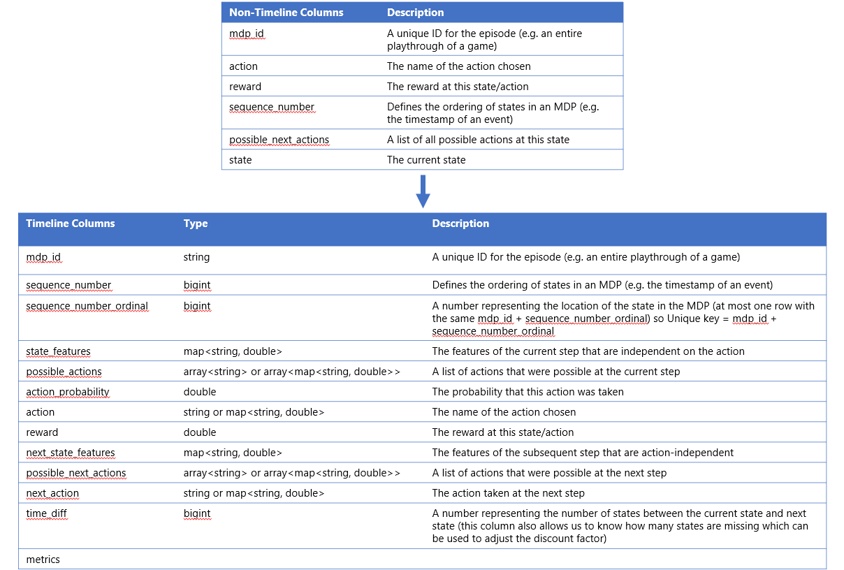
This will execute a Spark Job, run a query through Hive and return the results in a different file.
# Build timeline package (only need to do this first time)
mvn -f preprocessing/pom.xml clean package

# Clear last run's spark data (in case of interruption)
rm -Rf spark-warehouse derby.log metastore_db preprocessing/spark-warehouse preprocessing/metastore_db preprocessing/derby.log

# Run timelime on pre-timeline data
/usr/local/spark/bin/spark-submit \
  --class com.facebook.spark.rl.Preprocessor preprocessing/target/rl-preprocessing-1.1.jar \
  "`cat ml/rl/workflow/sample_configs/discrete_action/timeline.json`"

# Merge output data to single file
mkdir training_data
mv cartpole_discrete_timeline/part* training_data/cartpole_training_data.json

# Remove the output data folder
rm -Rf cartpole_discrete_timeline
After execution we can now watch the created file by running: head -n1 training_data/cartpole_training_data.json:
{
    "mdp_id": "31",
    "sequence_number": 5,
    "propensity": 1.0,
    "state_features": {
        "0": -0.029825548651835395,
        "1": 0.19730168855281788,
        "2": 0.013065490574540607,
        "3": -0.29148843030554333
    },
    "action": 0,
    "reward": 1.0,
    "next_state_features": {
        "0": -0.02587951488077904,
        "1": 0.0019959027899765502,
        "2": 0.00723572196842974,
        "3": 0.005286388581067669
    },
    "time_diff": 1,
    "possible_next_actions": [1, 1],
    "metrics": {
        "reward": 1.0
    }
}
Interesting here is that the Spark engine will allow us to utilize a distributed cluster running completely with CPU operations. The GPU operations will come in a later stage. Allowing us to completely utilize one cluster on HDFS and one cluster purely for the GPU calculations.
3. Normalization
To reduce noise and train our Neural Networks faster, we utilize "Normalization". Horizon includes a tool that automatically analyzes the training dataset and determines the best transformation function and corresponding normalization parameters for each feature.
To run this, the following command can be used:
python ml/rl/workflow/create_normalization_metadata.py -p ml/rl/workflow/sample_configs/discrete_action/dqn_example.json
Opening up the /ml/rl/workflow/sample_configs/discrete_action/dqn_example.json file we can see a similar config file as passed to the main function of our Gym Environment:
{
    "training_data_path": "training_data/cartpole_training_data.json",
    "state_norm_data_path": "training_data/state_features_norm.json",
    "model_output_path": "outputs/",
    "use_gpu": true,
    "use_all_avail_gpus": true,
    "norm_params": {
        "output_dir": "training_data/",
        "cols_to_norm": [
            "state_features"
        ],
        "num_samples": 1000
    },
    "actions": [
        "0",
        "1"
    ],
    "epochs": 100,
    "rl": {
        "gamma": 0.99,
        "target_update_rate": 0.2,
        "reward_burnin": 1,
        "maxq_learning": 1,
        "epsilon": 0.2,
        "temperature": 0.35,
        "softmax_policy": 0
    },
    "rainbow": {
        "double_q_learning": true,
        "dueling_architecture": false
    },
    "training": {
        "layers": [-1,
            128,
            64, -1
        ],
        "activations": [
            "relu",
            "relu",
            "linear"
        ],
        "minibatch_size": 256,
        "learning_rate": 0.001,
        "optimizer": "ADAM",
        "lr_decay": 0.999,
        "warm_start_model_path": null,
        "l2_decay": 0,
        "use_noisy_linear_layers": false
    },
    "in_training_cpe": null
}
So let's open up the ml/rl/workflow/create_normalization_metadata.py file where we can instantly see in its main method that it starts with a function called: create_norm_table.
The create_norm_table() method will take in the parameters (which is the json above) and utilize the norm_params, training_data_path, cols_to_norm and output_dir configs to create the normalization table.
This normalization table is build by checking the columns to normalize (which in the case of the json above is the column state_features) which will get the metadata through the get_norm_metadata() function. This function will start reading from our dataset and start sampling the features and its values. Once it collected enough samples (as defined by the norm_params["num_samples] configuration), it will continue.
4. Training the Model
Since everything is pre-processed now and the data is normalized, we are ready to start training our model. For this we can run the following command:
python ml/rl/workflow/dqn_workflow.py -p ml/rl/workflow/sample_configs/discrete_action/dqn_example.json
Which will utilize the dqn_workflow.py file that will choose the correct trainer to train its model. Running this will result in:
INFO:__main__:CPE evaluation took 0.23067665100097656 seconds.
INFO:__main__:Training finished. Processed ~3961 examples / s.
INFO:ml.rl.workflow.helpers:Saving PyTorch trainer to outputs/trainer_1543773299.pt
INFO:ml.rl.workflow.helpers:Saving Caffe2 predictor to outputs/predictor_1543773299.c2
INFO:ml.rl.caffe_utils:INPUT BLOB: input.1. OUTPUT BLOB:11
INFO:ml.rl.training.dqn_predictor:Generated ONNX predict net:
INFO:ml.rl.training.dqn_predictor:name: "torch-jit-export_predict"
op {
  input: "input.1"
  input: "1"
  input: "2"
  output: "7"
  name: ""
  type: "FC"
}
op {
  input: "7"
  output: "8"
  name: ""
  type: "Relu"
}
op {
  input: "8"
  input: "3"
  input: "4"
  output: "9"
  name: ""
  type: "FC"
}
op {
  input: "9"
  output: "10"
  name: ""
  type: "Relu"
}
op {
  input: "10"
  input: "5"
  input: "6"
  output: "11"
  name: ""
  type: "FC"
}
device_option {
  device_type: 0
  device_id: 0
}
external_input: "input.1"
external_input: "1"
external_input: "2"
external_input: "3"
external_input: "4"
external_input: "5"
external_input: "6"
external_output: "11"

INFO:ml.rl.preprocessing.preprocessor_net:Processed split (0, 4) for feature type CONTINUOUS
INFO:ml.rl.preprocessing.preprocessor_net:input# 0: preprocessor_net.py:287:Where_output0
5. Evaluating the Model
The model is trained, but how do we test it? This can be done through the included eval script for the cartpole experiment:
python ml/rl/test/workflow/eval_cartpole.py -m outputs/predictor_<number>.c2
def main(model_path):
    predictor = DQNPredictor.load(model_path, "minidb", int_features=False)

    env = OpenAIGymEnvironment(gymenv=ENV)

    avg_rewards, avg_discounted_rewards = env.run_ep_n_times(
        AVG_OVER_NUM_EPS, predictor, test=True
    )

    logger.info(
        "Achieved an average reward score of {} over {} evaluations.".format(
            avg_rewards, AVG_OVER_NUM_EPS
        )
    )


def parse_args(args):
    if len(args) != 3:
        raise Exception("Usage: python <file.py> -m <parameters_file>")

    parser = argparse.ArgumentParser(description="Read command line parameters.")
    parser.add_argument("-m", "--model", help="Path to Caffe2 model.")
    args = parser.parse_args(args[1:])
    return args.model
This will run our Gym Environment with the given model and return the reward score over x evaluation as a log line.
An example of this is:
INFO:__main__:Achieved an average reward score of 9.34 over 100 evaluations.
6. Visualizing via Tensorboard
Now the last step is to visualize everything through Tensorboard, which we can start as:
tensorboard --logdir outputs/
Which will spawn a process that binds to https://localhost:6006.
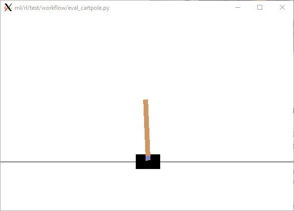
Rendering our Trained Model
Once we trained our model, we were able to visualize it through Tensorboard. However we also would like to be able to view the model running while evaluating it. To be able to start with this, first install the prerequisites + dependencies as shown here: How to run OpenAI Gym on Windows and with Javascript.
Another thing we now have to do is to change the eval_cartpole.py file and add render=True in the run_ep_n_times() method, making it look like this:
avg_rewards, avg_discounted_rewards = env.run_ep_n_times(
    AVG_OVER_NUM_EPS, predictor, test=True, render=True
)
When we now relaunch our evaluator through:
python ml/rl/test/workflow/eval_cartpole.py -m outputs/predictor_<number>.c2
We will be able to see our process spawn:


Comments ()