An introduction to Reinforcement Learning (RL)

So as we learned in the intro to Machine Learning, Reinforcement Learning is this technique where we have an agent who will take specific actions on an environment to try to reach an optimal state. But how can we illustrate this? Take a look at the following picture.

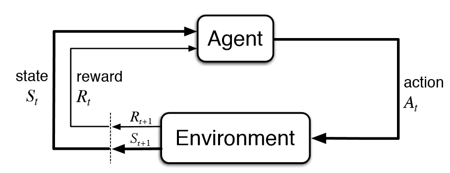
We can see here that an Agent will take a certain action $At$ to receive the reward $Rt$ at timestamp $t$. But what action should we take if we know the rewards? Well this is known as the Exploration/Exploitation Dilemma. For example, just think about having the choice between 100USD, 1.000USD or an unknown reward, which will you take? Will you take a risk and go for the unknown? or will you play safe and go for the 1.000USD?

Now let's go over our different elements in Reinforcement Learning that we will need in the further posts.

Basic Reinforcement Learning Elements

Environment

The environment its task is to define a world where an agent is able to interact with. It therefore has a basic loop that can be written like this:

1. Produce state $s$ and reward $r$

Where our state $s$ represents the current situation in the environment and the reward $r$ represents the scalar value being returned by the environment after selecting an action $a$.

Note: We will mostly use $at$, $rt$, $s_t$ showing at which timestep we are receiving these results.

Agent

Our agent needs to learn how to achieve goals by interacting with the environment. The basis to do this is by using a basic loop.

1. Sense state $s$ and reward $r$ from the environment
2. Select an action $a$ based on this state and reward

We do note here though that the action that our agent can take can be defined under two specific categories:

• Discrete: 1 of N actions (for example, left or down)
• Continuous: An action as a scalar/vector of a real value (for example, the amount we need to bend our leg to be able to walk)

Policy $\pi$

We want to achieve the best and shortest possible path towards the optimal state. Therefore we use a Policy $\pi$ that maps the actions to the states that we have to take. This can just as our action be categorized in two specific categories:

• Deterministic: Same action every time
• Stochastic: There is a probability of taking another action (example, we take action 1 70% of the time, and action 2 30% of the time)

To give you an example of a Stochastic Policy, take a look at the following:

|state $s$|action $a$|nextState $s^{'}$|reward $r$|probability| |-|-|-|-|-| |S1|A1|S2|-1|0.3| |S1|A1|S3|0|0.7| |S1|A2|S4|0|0.1| |S1|A2|S5|0|0.1| |S1|A2|S6|0|0.8| |S1|A1|S7|0|0.5| |S1|A1|END|1|0.5|

We can thus say that our policy is a function that is based on a state $s$ and an action $a$, or $\pi(s, a)$

Value function $V$

The value function is a complex something, it represents the goodness of state in the long run, which is calculated by our agent. Or in other terms What is the expected long term accumulation of reward.

Let's look at an example of this value function. In the game Tic-Tac-Toe, placing our X in the middle in the start of the game would increase our odds in winning. Therefore the Value Function for this position would return a higher value, than where we put our X somewhere else (see the example on the right).

$$ \begin{array}{c|c} High\,Value \ \hline \begin{array}{c|c|c} O & O & O \ \hline O & X & O \ \hline O & O & O \ \end{array} \end{array} \,\,\, \begin{array}{c|c} Low\,Value \ \hline \begin{array}{c|c|c} O & O & O \ \hline X & O & O \ \hline O & O & O \ \end{array} \end{array} $$

We have two different value functions:

• State-Value Function $V^\pi(s)$: Value of state $s$, when following policy $\pi$
• It gives the expected return when starting from state $s$ and following our policy $\pi$ forever.
• $V^{\pi}(s) = E{\pi}[Rt|s_t = s]$
• Action-Value Function $Q^\pi(s,a)$: Value of state $s$, taking action $a$, and thereafter following policy $\pi$ forever.
• It gives the expected return of taking action $a$ in state $s$, given our policy $\pi$
• $Q{\pi}(s, a) = E{\pi}[Rt|st = s, a_t = a]$
• Note: This is also commonly referred to as the Q-value

Tasks

in Reinforcement Learning, we have two sorts of tasks. Episodic ones and Continuing ones:

• Episodic: Tasks that come to an end (example: tic-tac-toe, pac-man, …)
• Continuing: Tasks that never end (example: tuning a heating system)

Fundamental Challenges

Reinforcement Learning has four key challenges that will result in a good or bad performing algorithm. All of those challenges can be isolated in their own black box environment and researched independently.

1. Representation: How to represent the states, actions and outcomes?
2. Generalization: How can we make the RL algorithm behave well in unseen situations?
3. Temporal Credit Assignment: How can we find the actions in a sequence that contributed the most to a certain outcome?
4. Exploration: Is there an action that we didn't try yet, that could lead to a better outcome?

More about this in the following posts.